(the number of current visitors is automatically updated every 4 minutes)

If you want to share information about this web page...
Logistic regression is a common statistical technique, and reading this webpage will help you understand more about it. This page also contains advice if you want to analyze your own data using logistic regression.
You will understand this webpage best if you have first read the pages Introduction to statistics, Observations and variables, Inferential statistics, Covariation and Correlation and regression.
The concept of logistic regression
Logistic regression is a kind of linear regression where the dependent variable (Y) is not continuous (does not have an order with equidistant scale steps). All variables are transformed using the function for natural logarithms. A standard linear regression is made where the outcome is transformed back using the inverse of natural logarithms (e.g. the exponential function). The beta coefficients produced by the logistic regression is often transformed to odds ratios. Logistic regression creates equations similar to the equations created by standard linear regression:
Standard linear regression equation: Y = a + b1x1 + b2x2 + b3x3
Binary logistic equation: Log-odds = a + b1x1 + b2x2 + b3x3
X represents the different independent variables and b their respective beta coefficients.
The landscape of logistic regression models
Possible different situations within the concept of logistic regression are:
| One dependent and one independent variable (one “y” and one “x”) | More than one independent variable (one “y” and multiple “x’s”) | More than one dependent variable (multiple “y’s” and one or several “x’s”) | |
|---|---|---|---|
| The dependent variable is binary and the sample consists of independently chosen observations. | Unconditional simple logistic regression = unconditional unadjusted logistic regression = unconditional binary logistic regression (=bivariate logistic regression) | Unconditional multiple logistic regression = unconditional multivariable logistic regression = unconditional adjusted logistic regression | Unconditional multivariate logistic regression |
| The dependent variable is binary and the sample consists of independently chosen matched pairs. | Conditional simple logistic regression = conditional unadjusted logistic regression | Conditional multiple logistic regression = conditional multivariable logistic regression = conditional adjusted logistic regression | Conditional multivariate logistic regression |
| The dependent variable is categorical with more than two categories / values and the sample consists of independently chosen observations. | Multinomial simple logistic regression (=multiclass simple logistic regression) | Multinomial multiple logistic regression (=multiclass multiple logistic regression) | Multinomial multivariate logistic regression |
| The dependent variable is ordinal (has an order but not equidistant scale steps) and the sample consists of independently chosen observations. | Ordered simple logistic regression = ordinal simple logistic regression = ordered simple logit model | Ordered multiple logistic regression = ordinal multiple logistic regression = ordered multiple logit model | Ordered multivariate logistic regression = ordinal multivariate logistic regression = ordered multivariate logit model |
There is a confusion where many incorrectly write multivariate logistic regression when they in fact have only one “y” and multiple “x’s”.
The rest of this page will focus on unconditional binary logistic regression because this is the most commonly used logistic regression. First look at this brief introduction by Josh Starmer:
It’s Not About Transport: The Real History of Logistic Regression
Malthus argued in his essay published in 1798 that while food production grows linearly (1,2,3,4,5…), population grows exponentially (1, 2, 4, 8, 16…), leading inevitably to famine, disease, or war . In the 1830s the Belgian mathematician Pierre François Verhulst, who sought to challenge Malthus’s terrifying prediction discovered that populations don’t explode infinitely but naturally brake as resources dwindle, tracing an elegant “S” shape he mysteriously named the “logistic” curve.
Verhulst’s work lay forgotten until 1920, when Raymond Pearl and Lowell Reed rediscovered it to model US population growth, controversially declaring it a universal law of biology. They championed it as a universal law of growth, applying it to everything from fruit flies to nations, sparking a scientific frenzy. But there was a problem: no one knew how to calculate the curve’s parameters with precision until the British genius Sir Ronald A. Fisher stepped in. Fisher developed the method of “Maximum Likelihood,” providing the rigorous mathematical engine required to fit these complex models to real data.
For nearly a century, this curve was merely a demographic tool, until 1940s statisticians like Joseph Berkson saw a hidden brilliance in its geometry. Berkson realized this “S” shape was perfect not for counting crowds, but for modeling probabilities—transforming linear data into binary “yes or no”.
Why logistic regression is practical
Unconditional binary logistic regression is perfect for evaluating the correlation between any variable and a dichotomous dependent variable. Many group comparisons should preferably be analysed using logistic regression rather than a chi-square or t-test. The reason why logistic regression has an advantage over simpler group comparisons, such as chi-square and t-test, is:
- The ability to adjust for other covariates. The importance of each variable can be determined while simultaneously adjusting for the influence of other variables. This usually gives a better reflection of the true importance of a variable.
- There are techniques to reduce the number of variables so only the relevant ones remain. This reduces the problem of multiple testing.
Let me explain the latter point using an example. Assume we want to know which variables differ between two groups: those who have experienced an illness compared to those who have not (or, for example, those who answer ‘yes’ to a question compared to those who answer ‘no’). Also, assume that we want to investigate 50 different variables, some being categorical while others are continuous. Using a chi-square or t-test to compare the two groups would result in 50 p-values, some below and some above 0.05. However, a p-value below 0.05 can occur by chance. To compensate for the possibility of finding statistical significance by pure chance, we need to lower the threshold for what we consider a significant finding. There are multiple ways of doing this. For instance, using a simple Bonferroni adjustment would mean that only p-values below 0.001 should be considered statistically significant (0.05 / 50 = 0.001). A consequence of this is that very few, or none, of the calculated p-values might be considered statistically significant.
Using logistic regression, as described below, mitigates this problem. We would first use a technique as a sorting mechanism to decide which variables to include in the second step: a multiple regression. A common scenario is to start with 50 independent variables. It is reasonable to believe that only 2–5 variables will remain statistically significant in the final model. Assume that we finally end up with 5 p-values (and odds ratios). According to Bonferroni, any p-value below 0.01 can now be considered statistically significant (0.05 / 5 = 0.01). Consequently, we have substantially reduced the problem of multiple testing.
The two arguments for using multiple logistic regression (when the dependent variable is dichotomous) rather than a simple group comparison would also apply to multiple standard linear regression (if the dependent variable is continuous) and multiple Cox regression (if a time factor is the dependent variable).
How to do logistic regression in practice?
Look at this video by Steve Grambow explaining the math behing unconditional binary logistic regression. You don’t need to remember it but seeing this video gives you a deeper understanding of what it is all about.
Prerequisites your data must meet
- All your observations are chosen independently. This means that your observations should not be grouped / clustered in a way that can have an influence on the outcome. (You can have grouped / clustered observations and adjust for this. However, that is a bit complicated in logistic regression and cannot be done in all statistical software)
- You have enough observations to investigate your question. The number of observations you need should be estimated in advance by doing a sample size calculation.
- The dependent variable is a binary class variable (only two options). Usually this variable describes if a phenomenon exists (coded as 1) versus does not exist (coded as 0). An example can be if a patient has a disease or if a specified event happened.
- Categorical independent variables must be mutually exclusive. This means it must be clear if an observation should be coded as a
0
or as a1
(or anything else if the categorical variable has more than two values). - There should be a reasonable variation between the dependent variable and categorical independent variables. You can check for this by doing a cross-table between the outcome variable and categorical independent variables. Logistic regression might be unsuitable if there are cells in the cross-table with few or no observations.
- The independent variables do not correlate to much to each other in case you have more than one independent variable. This phenomenon is labelled multicollinearity. You should test for this when you do a multiple binary logistic regression.
- Any continuous independent variables must have a linear correlation with the logit or the binary dependent variable. The model constructed will not fit well if there is a non-linear correlation such as a polynomial correlation. You do not need to test for this before doing the logistic regression but checking this should be a part of the procedure when you do the regression.
Ensure that all variables are coded to facilitate clear interpretation of the results. Special attention should be paid to categorical variables to ensure the coding scheme is sensible. For instance, when analyzing ethnicity, you must determine whether to retain a distinct option for every alternative or to merge them into broader groups. This decision depends on your research focus and the nature of the data. It is often worth considering whether merging multiple categories into just two groups might simplify the interpretation of the outcome.
Necessary preparations
- Data cleaning: Do a frequency analysis for each variable, one at the time. You are likely to find some surprises such as a few individuals with a third gender or a person with an age that is unreasonable or more missing data than you expect. Go back to the source and correct all errors. Recheck all affected variables after correction by doing a new frequency analysis again. This must be done properly before proceeding.
- Investigate traces of potential bias: Have a look at the proportion of missing data for each variable. There are almost always some missing data. Is there a lot of missing data in some variables? Do you have a reasonable explanation for why? Can it be a sign that there is some built in bias (systematic error in the selection of observations/individuals) in your study that may influence the outcome?
- Adjust independent variables to facilitate interpretation: Quite often a few variables needs to be transformed to a new variable. It is usually easier to interpret the result of a logistic regression if the independent variables are either a binary or a continuous variable. A class variable with several options might be better off either being merged to a binary variable or split into several binary variables. For continuous variables it may sometimes be easier to interpret the result if you change the scale. A typical example of the latter is that it is often better to transform age in years to a new variable showing age in decades. When you want to interpret the influence of age an increase in one year is often quite small but an increase in age of one decade is usually more clinically relevant (at least for adults). You can see in table 4 in the publication by Hargovan et al that the odds ratio for age is provided per decade and not per year to make the odds ratio more meaningful. Another example is systolic blood pressure where it might be sensible to calculate odds ratios for a change in 10mmHg rather than 1mmHg. Many laboratory investigations (blood or urine test) may also enhance interpretation by changing the scale from a small unit to a larger.
- Decide strategy: Do unadjusted binary logistic regression if you have only one independent variable. However, if you have multiple independent variables then you need to choose a strategy for including independent variables in your analysis. There are a few different possibilities to do this. The first approach (4a) is the best. However, that is not always possible so you may have to use another strategy.
- Decide, due to logical reasons / theories (expert advice), to use a set combination of independent variables. The number of independent variables should not be too many, preferably less than 10. This would be the preferred method if you have a reasonably good theory of how to link the variables to each other.
- Do a multiple regression with all available independent variables without having any theory if these variables are meaningful. This may work if you only have a few variables. If you have many variables it is likely to result in a final model containing many useless variables that can be considered as clutter. Hence, avoid doing this.
- If you have many independent variables and no theory of which ones are useful you may let the computer suggest which variables are relevant to include. This would be considered going on “a fishing expedition”. You can read more about this below.
Building a multivariable model – based on predetermined theory
Building a logistic model where you, rather than a software program, decides what to include is the preferred method. The video below describes how to build such a model, as described in 4a above, in SPSS:
Building a multivariable model – fishing expedition
This describes how to build a model, as described in 4c above. This procedure can start with many independent variables (no direct upper limit) and eliminate the ones of lesser importance. This procedure is also labelled as a fishing expedition. Nothing wrong in that but, important to maintain a suspicion towards statistically significant findings that seems peculiar. Many statistical software packages have automated procedures for this. This exists as several different methods:
- Forward inclusion/selection: Can be used if you have more variables than observations. Once a variable is added, it usually stays. It might pick variable A first because it looks good alone, but it misses the fact that variable B and C together would have been a much better predictor. It often fails to capture complex relationships that only appear when multiple variables are present. The methods below are better.
- Backwards elimination: Useful if you have more observations than variables.
- Stepwise regression: It is a hybrid. It usually starts like forward selection (adding variables), but at every step, it checks backward to see if any variable that was previously added has now become insignificant (perhaps because the new variable explains the same thing better). It fixes the main flaw of forward selection. If variable A was added early but became useless once variable C was added, Stepwise regression will throw variable A back out. It is more flexible and better than “Forward inclusion/selection” and “Backwards elimination”. Look at this video by Brandon Foltz that introduces this concept: https://www.youtube.com/watch?v=An40g_j1dHA.
- Regularization techniques such as LASSO regression, Ridge regression and Elastic Net. These methods can also be labelled as “penalized regression or “regularized regression“. Spetwise regression has a risk of overfitting your model to your unique observations. Regularization techniques solves this problem by by introducing a penalty for complex models. They are now considered superior to conventional stepwise regression . Of these models Elastic net is perhaps the best one and it can be performed in R, STATA and SPSS (the more modern versions of SPSS). Read more about this on the page regularized regression.
Some practical advice:
- If you insists on using a stepwise regression then you must first check all independent variables for zero order correlations. This means checking if any of the independent variables of potential interest correlates strongly to each other. If that is the case then you must make a choice before proceeding. There is no clear cut definition of a “strong correlation”. I suggest that two independent variables having a Pearson (or Spearman) correlation coefficient above +0.7 or below -0.7 with a p-value <0.05 should be considered as being too correlated. If that is the case then you need to omit one of them from further analysis. This choice should be influenced on what is most practical to keep in the further analysis (what is likely to be more useful). The best way to do this in SPSS is to do a standard multivariate linear regression and in the Statistics button tick that you want Covariance matrix and Collinearity diagnostics. Ignore all output except these two outputs.
- if you use regularization techniques you don’t have to worry about correlation between independent variables. These regularization regressions are usually better at choosing how to retain variables than if we ourselves do it (unless we have a valid theory of which variables to include).
Evaluate your logistic model
Models are often evaluated in respect of their ability to separate (or correctly diagnose) individuals (labelled discrimination) or wether predicted probabilities are similar to observed outcome (labelled calibration) . Good discrimination is very important when evaluating a diagnostic model while good calibration is important when evaluating models aimed to predict a future event . There are also estimates of the overall performance of the new model. Discrimination, calibration and overall performance are somewhat linked so an excellent model usually have high discrimination, calibration as well as a good overall performance. The most common measures to estimate the value of a model, adapted from Steyerberg et al :
- Overall performance:
- Cox and Snell R Square is a kind of pseudo R square statistics. A higher value is better.
- Nagelkerke R square is an adjusted version of the Cox and Snell R square. Many statistical software packages delivers this if you tick the right box when you command the software to do logistic regression. It describes how well variation in the the dependent variable is described by variation in the independent variables. Zero means that the new model is useless and 1.0 that it is absolutely perfect. Thus, the higher the better. A simple and reasonable (although not entirely correct ) translation is that a value of 0.10 means that roughly 10% of the variation in the dependent variable is associated with variations in the included independent variables. If the Nagelkerke is below 0.1 it means your model only explains a small amount of the variation in the dependent variable. A good model would typically have a Nagelkerke R square of >0.2 and a value of >0.5 indicates an excellent model.
- Discrimination:
- Sensitivity and Specificity and predictive value of test are calculated for a given cut of of the probability for having the outcome. These values can be presented for any cut off but the most commonly used cut off of is a 50% probability of having the outcome.
- An extension of sensitivity and specificity is a Receiver operating curve analysis (ROC) analysis. It calculates the sensitivity and specificity for all possible cut offs in probability for the outcome. Look at the figure for Area under the curve (AUC). This usually goes from 0.5 (the model is as good as pure chance) to 1.0 (the model is perfect). AUC is also labelled concordance statistics or “c-statistics”. An AUC between 0.50-0.60 indicates that your model is hardly any better than pure chance (which is bad). An AUC above 0.80 usually indicates your model is quite good and above 0.90 is absolutely excellent. ROC analysis is a separate analysis requiring you to save the estimated probability for the event for each observation when you do the logistic regression.
- Discrimination slope.
- Calibration:
- The Omnibus Tests of Model Coefficients (provided by IBM SPSS). A low p-value indicates a good calibration.
- Hosmer and Lemeshow test investigates if the new model describes the observations better than pure chance. A low p-value indicates that it is not better than pure chance while a high p-value says your model has good calibration. This test is too sensitive if you have large data sets. Many statistical software packages delivers this if you tick the right box when you command the software to do logistic regression.
- Calibration slope.
- Reclassification:
- Reclassification table.
- Reclassification calibration.
- Net Reclassification Index (NRI)
- Integrated Discrimination Index (IDI)
- Clinical usefulness
- Net Benefit (NB)
- Decision curve analysis (DCA)
The most commonly used measures of model validity are Nagelkerke R square, Receiver operating curve analysis (ROC) analysis and Hosmer and Lemeshow test. Measures to estimate “Reclassification” and “Clinical usefulness” are more recent inventions and hence not yet used a lot . All of the above tests for model validation can be applied slightly differently:
- Most often you would use 100% of your observations to create your model and then use the same 100% to validate your model. This is labelled internal validation and should always be presented.
- You can use 70-75% of your observations to construct your model and 25-30% of them to test your model. This might be a good idea if you have many observations. This is sometimes labelled split-sample validation.
- The ultimate test is to apply your model to another set of observations obtained from another site / context . Validating your model in this new set of observations estimates how useful your model is outside where it was constructed. This is labelled external validation. Excellent models would have a good overall performance with high discrimination and calibration in both internal and external validation. Achieving this is very rare.
Interpreting logistic regression results
Logistic regression is about calculating how one or several independent variables are associated with one dependent variable, the latter always being dichotomous. For each of the variables you are likely to have some missing data. If you do a multivariate logistic regression (more than one independent variable) these missing data vill accumulate. Hence, you may have 10% missing data in one variable and 10% in another. However, the 10% of observations having missing data in one variable may be different observations than the observations missing in another variable. Hence, 10% missing data in one variable and 10% missing in another may in worst case add up to 20%, and so on. For this reason it is important to look at the total proportion of observations that could not be used in this multivariate logistic regression.
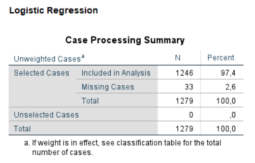
Let us look at an example where we want to see how gender, age, smoking and use of use of moist snuff (oral tobacco) correlate to perceived health . See image above where a total of 2.6% of observations could not be used because they had missing data in at least one of the variables. A large proportion of missing data is alarming and could potentially be a sign of some systematic problem that needs to be clarified. 2.6% as in this example is fine.
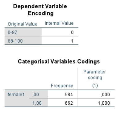
In this example perceived health is the dependent variable and is measured with the dimension physical functioning in the quality of life survey SF-36. The dependent variable is an ordinal scale but in this example it is dichotomised at the level of the average percieved health for the healthy Swedish population (the average for the Swedish population in this age group is 87). Hence, a 1 means better than average health while a 0 means equal to or lower than average health (see image).
In the image we can see that the dependent variable is from the start measured by an ordinal scale being transformed into a new variable by introducing a cut off. It is important to understand that variables originally being 88-100 will be coded as 1 and values 0-87 as 0 in this regression. It mean the odds ratios will predict a higher value of the dependent variable rather than the other way around. We can also see that for gender the software chose to code female gender as 1 and male as 0. This means the odds ratio for the independent variable gender will give the odds ratio for being female is associated with having the higher range of the score in the dependent variable.
It is essential to check how the dependent and independent variables are coded. Independent variables being measured with an interval or ratio scale are usually automatically coded with their value. Hence, a value of 5 is 5 in the regression analysis. This may not be the case with variables measured with the nominal scale. You always have to look up how these categorical variables are coded by your software because it decides how the result should be interpreted.
The logistic regression results in an odds ratio for each of the independent variables. The odds ratio can be anything from 0 and upwards to infinity. Odds ratio can never be below zero.
- Odds ratio = 1.0: means the independent variable is not correlated to the variation of the dependent variable.
- Odds ratio > 1.0: means an increase in the independent variable is associated with an increase in the dependent variable (more likely the outcome is a 1 rather than a 0).
- Odds ratio < 1.0: means an increase in the independent variable is associated with a decrease in the dependent variable (more likely the outcome is a 0 than a 1).
Have a look at the image below. B is the beta-coefficient (similar to the one in standard linear regression). The beta coefficient can assume any value from negative infinity to plus infinity. The B-coefficient is also transformed to an odds ratio and this software (SPSS) labels it “Exp(B)”. The Odds ratio will be 1.0 when the B coefficient is zero. The two columns to the right are the 95% confidence interval for the odds ratio. From this we can make the following interpretations:
- Female gender is associated with a decreased chance of having high score (odds ratio is below 1.0).
- Increasing age is associated with a decreased chance of having high score (odds ratio is below 1.0). The age is here stated in decades so we get the odds ratio for an increased age of one decade.
- Smoking is associated with a decreased chance of having high score (odds ratio is below 1.0). Smoking is here stated in 10th of pack years so we get the odds ratio for an increase of 10 pack years.
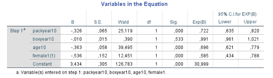
The study in this example showed that poorer perceived health was associated with smoking, higher age and being a woman where the latter had the lowest odds ratio for havinbg a good health.
Below is a video showing another example of a logistic regression and how to interpret the result:
Reporting the results of a logistic regression
Results from multivariable binary logistic regression should always be presented in a table where the first column lists all independent variables evaluated, the following columns presents the outcome of the regression. However, if data are suitable they may also lend themselves to be presented as a user friendly look up table or probability nomogram. Look up tables might be a good option if you only have dichotomous independent variables remaining in the final model. Probability nomograms are often a good option if you have only one continuous variable remaining in the final model (see examples below). If you end up in a final model with multiple continuous variables the options are:
- Simply present data in a table (see practical examples below). This must be done anyway and it is not always a good idea to do more.
- Investigate the consequences of dichotomising all independent continuous variables except one. Sometimes the explanatory power of the model (measured by Nagelkerke R-square and AUC) only goes down marginally with a few per cent. This price might be acceptable to enable presenting a complicated finding in a much more user friendly way. If that is the case it enables you to create a user friendly probability nomogram. This is often worth investigating.
- Create a complicated probability nomogram (unlikely to be user friendly).
- Create a web based calculator where the user puts in information and a probability is calculated or make a phone app that does all calculations when the user puts in data. This is likely to work fine even if you have several independent variables measured by a continuous scale.
Practical examples of presenting the outcome from multivariate logistic regression:
- Antimicrobial resistance in urinary pathogens among Swedish nursing home residents : Table 4 shows how to combine the outcome of several bivariate (=univariate) logistic regressions and a following multivariable logistic regression in a single table.
- Prognostic factors for work ability in women with chronic low back pain consulting primary health care: a 2-year prospective longitudinal cohort study : Table 4 shows how to combine the outcome of several bivariate (=univariate) logistic regressions and a following multivariable logistic regression in a single table. This publication also demonstrate how the outcome in a multiple binary logistic regression can be presented as probability nomograms (Figure 2). The latter is recommended if your final model only contains one continuous variable and a limited number of categorical variables. Predictive nomograms can be constructed also for models having more than one continuous variable but they tend to be complicated and less intuitive.
- Predicting conversion from laparoscopic to open cholecystectomy presented as a probability nomogram based on preoperative patient risk factors : Table 2 shows how to combine the outcome of several bivariate (=univariate) logistic regressions and a following multivariable logistic regression in a single table. This publication also demonstrate how the outcome in a multiple binary logistic regression can be presented as probability nomograms (Figure 1-4). This manuscript also clearly states that the bivariate regressions are only considered as a sorting mechanism and the outcome of them are not considered as a result. It states that only the remaining variables in the multivariable regression is the actual result (and adjust the level of significance accordingly).
- Predicting the risk for hospitalization in individuals exposed to a whiplash trauma : In this example the final regression model contains no continuous variables. Hence, a lookup-table is constructed (Table 3). Table 3 was constructed by ranking the predicted probabilities of all possible permutations of the final predictors.
More information
- Restore – Module 4: Binary Logistic Regression (I recommend you have a look here)
- Julie Pallant. Logistic regression. in SPSS survival manual. (Extremely useful if you use SPSS)
- Recommendations for the Assessment and Reporting of Multivariable Logistic Regression