(the number of current visitors is automatically updated every 4 minutes)

If you want to share information about this web page...
This web-page describes level of significance and how this relates to p-values. These concepts are sometimes mixed up and reading this page will enable you to understand the difference. The page also contains online calculators that will help you.
You will understand this page best if you have read Introduction to statistics and Inferential statistics.
The difference between level of significance (alpha) and the p-value
A low p-value indicates that the observed result, or a more extreme one, would be unlikely under the null model. We reject the null hypothesis in favor of an alternative hypothesis, without this implying that the alternative hypothesis has been assigned a probability. But exactly how low must the p-value be for us to take this step? This threshold should be determined from case to case and is known as the level of significance, or alpha.
We use inferential statistics to calculate a p-value. The next step is to compare this calculated p-value against our predetermined level of significance (alpha). If the p-value is below alpha, we reject the null hypothesis and consider the alternative hypothesis to be the most plausible. Conversely, if the p-value is higher than alpha, we cannot reject the null hypothesis; our results do not provide enough evidence to contradict it..
By tradition, alpha is most often set to ≤0.05. Therefore, a p-value of 0.045 would be classified as statistically significant, while a p-value of 0.055 would not. However, it is crucial to remember that this ≤0.05 threshold is not black and white. In reality, findings of p=0.045 and p=0.055 are statistically very similar. Because of this, exact p-values should always be reported, rather than simply stating whether a finding was “significant” or not.
In summary: The level of significance (alpha) is a fixed limit determined by the researcher, usually in advance. It does not depend on our observations and is not calculated; rather, it is a conscious decision based on the safety margin needed to avoid making a Type I error (a false positive). The p-value, on the other hand, is calculated from the observed data using a specified statistical test and model assumptions.
The level of significance and pure chance
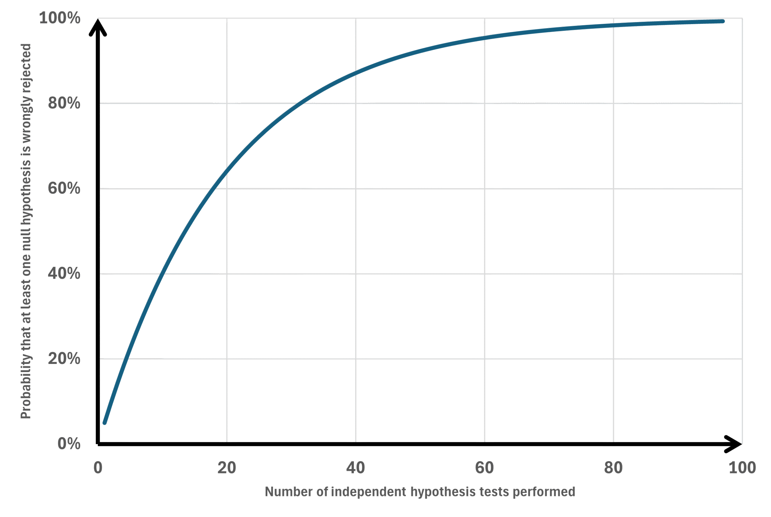
Assume we want to know which variables differ between two groups, those who have experienced an illness compared to those who have not (or it could be those who say yes to a question compared to those who say no). Also assume that we want to investigate 50 different variables, some being categorical while others are continuous. Using chi-square or t-test to compare the two groups would result in 50 p-values, some below and some above 0.05. However, a p-value ≤0.05 can occur by pure chance without representing a real difference between groups. The probability to wrongly reject the null hypothesis (believe that a low p-value represents something else than pure chance) increases the more tests we do (Figure 1).
Deciding the level of significance
When multiple p-values, within a defined family of p-values, are presented we should consider adjusting the significance threshold or otherwise controlling multiplicity. This is most important when making confirmatory claims but should also be considered in exploratory analysis. There are different methods to do this.
Family-Wise Error Rate (FWER) and False Discovery Rate (FDR)
Family-Wise Error Rate (FWER) is the probability of making at least one Type I error — that is, at least one false positive — across a family of statistical tests. In simpler terms: If you run several hypothesis tests, FWER is the chance that one or more of them incorrectly appears statistically significant just by chance (Figure 1). If all m null hypotheses are true and the tests are independent, the chance of at least one false positive is: 1-(1-alpha)^m (m=number of statistical tests). For example we make 20 statistical tests the chance of making at least one type I error is:
In this example it would be 64% chance of having at least one statistical test being false positive. FWER is concerned with controlling the probability of any such false discovery in the whole set of tests. FWER is stricter than the False Discovery Rate (FDR):
- FWER controls the chance of making any false positive.
- FDR controls the expected proportion of false positives among the statistically significant findings.
Overview of “universal adjusters” of the level of significance
| Method | Description | Advantage | Disadvantage |
|---|---|---|---|
| The Bonferroni method | Controls the Family-Wise Error Rate (FWER). Keeps the chance of making even one false positive at or below your chosen level of significance (such as ≤5%). For adjusted p-values, Holm-Bonferroni is usually preferable to unmodified Bonferroni. | Very simple to understand. Does not require that each test is independent. | “Very conservative” making it hard to find statistical significance if you calculate many p-values. |
| The (Dunn-)Šidák correction | Controls the Family-Wise Error Rate (FWER). Keeps the chance of making even one false positive at or below your chosen level of significance (such as ≤5%). Never use this method (better to use one of the below recommended methods). | Slightly less conservative than Bonferroni’s method. However, the difference is very small and this method is, like Bonferroni’s method likely to miss relevant findings. | Less easy to understand. Also requires that every single one of your 20 tests is completely independent of the others (which is often not the case in reality). |
| The Holm-Bonferroni method | Controls the Family-Wise Error Rate (FWER). Keeps the chance of making even one false positive at or below your chosen level of significance (such as ≤5%). Suitable for confirmatory research. | Less conservative compared to Bonferroni’s method meaning that the chance of finding a true statistical significance is higher than if you use Bonferroni’s method. Does not require that each test is independent. | It is still relatively conservative. If you are doing hundreds of tests, it will still wipe out a lot of potentially valid discoveries. |
| The Holm-Šidák correction | Controls the Family-Wise Error Rate (FWER). Keeps the chance of making even one false positive at or below your chosen level of significance (such as ≤5%). Suitable for confirmatory research. | Less conservative compared to Šidák correction meaning that the chance of finding a true statistical significance is higher than if you use Šidák correction. Does require that each test is independent. | Thr requirement for tests being completely indeopendent is the main disadvantage. |
| The Benjamini-Hochberg procedure | Instead of controlling the chance of making any false positive, this method controls the False Discovery Rate (FDR) meaning it accepts a small, known percentage of false positives in exchange for a much higher chance of discovering true significant differences. Suitable for exploratory research. | Massively more statistical power than any of the above methods. It is the gold standard for exploratory data analysis where you are screening dozens or hundreds of variables to see what looks promising. You use BH when you want to cast a wide net to find leads for future, more targeted research. Does not require complete independence under many common positive-dependence settings (however, under arbitrary dependence, Benjamini–Yekutieli or other methods may be more appropriate). | You may get some false positive findings, but their expected proportion among rejected hypotheses is controlled. |
The Bonferroni Method
This simple method means that we divide the desired overall level of significance (often 0.05) with the number of p-values calculated. In an example with 50 p-values calculated a Bonferroni adjustment means that only p-values ≤0.001 should be considered as statistically significant which may be difficult to achieve. Hence, Bonferroni’s method is not suitable if you calculate many p-values. For adjusted p-values, Holm-Bonferoni is usually preferable to unmodified Bonferroni because it controls FWER and is less conservative. Bonferroni remains useful in some contexts, especially for simultaneous confidence intervals ( se below).
The (Dunn-) Šidák correction
The standard Bonferroni correction sets the threshold for all tests at simply α/m. The Šidák correction uses an exact formula:
The Šidák threshold is slightly more forgiving. For example, with α = 0.05 and m = 10 tests the level of significance becomes 0.005 for Bonferroni and for Šidák 0.005116. So, Šidák is undeniably slightly more powerful than standard Bonferroni.
Holm-Bonferroni doesn’t just use one threshold; it adjusts dynamically (se below). If we pit single-step Šidák against step-down Holm-Bonferroni for 10 independent tests, here is what happens: For the very first (smallest) p-value: Šidák wins by a microscopic margin (0.005116 vs Holm’s 0.005000). For the second p-value: Holm’s threshold is now α/9 = 0.00555, which is already higher (more forgiving) than Šidák’s static 0.005116. For the third p-value: Holm’s threshold jumps to α/8 = 0.00625, further beating Šidák. Because Holm’s sequential thresholds quickly become much larger than Šidák’s single fixed threshold, Holm-Bonferroni will generally correctly reject more null hypotheses overall.
The Holm-Bonferroni Method
Controls the Family-Wise Error Rate (FWER) just like the standard Bonferroni, meaning it keeps the chance of making even one false positive at or below your chosen level of significance (such as ≤5%). Instead of treating every test the same, Holm-Bonferroni uses a “step-down” approach. It is essentially a smarter, less punishing version of the standard Bonferroni correction. The procedure is step by step:
- Rank your p-values: Order all your p-values from smallest (most significant) to largest (least significant).
- Apply a sliding threshold: Instead of dividing your alpha (foe example 0.05) by the total number of tests done for every single test, the threshold changes depending on the rank of the p-value. The formula for the adjusted threshold for the i-th ranked p-value is:
(Where alpha is 0.05, m is the total number of p-values calculated, and i is the rank of the p-value). - The Step-Down: For your smallest p-value, the threshold is exactly the same as the one calculated using the standard Bonferroni method. If your p-value is equal to or below this, it is significant. For your second smallest p-value, the threshold becomes slightly easier to achieve compared to the one calculated by the Bonferroni method. You then continue down the list. With each step, the threshold becomes larger (easier to achieve) compared to the threshold calculated by the Bonferroni method. As soon as you encounter a p-value that is larger than its calculated threshold, you stop. That variable, and all variables following it on the list, are declared statistically non-significant.
In a “Step-Down” procedure like Holm-Bonferroni, the p-values function like a series of gates. To reach the final gate, you must first pass through all the preceding ones. When the calculator encounters the first non-significant value, it closes the door completely. According to the rules of Holm-Bonferroni, that p-value and all subsequent p-values are then declared non-significant—regardless of how small they might be in relation to their own theoretical thresholds. This is the “penalty” inherent in Holm-Bonferroni: if one link in the chain breaks, the rest of the tests fall with it to protect against false positives.
Holm-Bonferroni calculator
The Holm-Šidák method
If your tests are strictly independent, Holm-Šidák is often the best choice. Both Holm-Šidák and Holm-Bonferroni use the exact same “step-down” algorithm (sorting p-values and making the threshold progressively easier to pass). The difference is entirely in the math formula they use at each step:
Because the Šidák formula calculates the exact probability for independent events rather than an approximation, its threshold is always slightly larger (more forgiving) at every single step. Therefore, Holm-Šidák will always have equal or greater statistical power than Holm-Bonferroni.
(A calculator for Holm-Šidák is under construction)
The Benjamini-Hochberg Procedure
Controls the expected proportion of the False Discovery Rate (FDR). This is a massive shift in statistical philosophy. Instead of trying to guarantee zero false positives, the BH procedure accepts that false positives will happen. Its goal is to control the expected percentage of your “significant” findings that are actually false. If you set FDR to 0.05, the procedure aims to keep the expected proportion of false discoveries among rejected hypotheses at or below 5%, under its assumptions. In any single study, the actual proportion can be higher or lower. The procedure is step by step:
- Rank your p-values: Order them from smallest on top to the largest at the bottom of the list.
- Calculate a critical value for each p-value: The threshold grows much faster than in the Holm-Bonferroni method. The formula is:
Critical Value = (i/m) * Q
(Where i is the rank, m is total number of p-values calculated, and Q is your chosen False Discovery Rate, usually 0.05). - The Step-Up: You look at your list and find the largest p-value that is smaller than its corresponding critical value. That variable, and every variable ranked smaller than it, is declared statistically significant.
The step-up procedure might be a bit diffficult to grasp so let us look at an example. In the calculator below, keep alpha at 0.05, and enter the following p-values: 0.060, 0.039, 0.035, 0.015, 0.005. This is how each p-value should be ranked and compared with its corresponding critical value:
- Rank 1:
0.005(Critical Value: 1/5 * 0.05 = 0.010) -> Passes (0.005 < 0.010) - Rank 2:
0.015(Critical Value: 2/5 * 0.05 = 0.020) -> Passes (0.015 < 0.020) - Rank 3:
0.035(Critical Value: 3/5 * 0.05 = 0.030) -> Fails (0.035 > 0.030) - Rank 4:
0.039(Critical Value: 4/5 * 0.05 = 0.040) -> Passes (0.039 < 0.040) - Rank 5:
0.060(Critical Value: 5/5 * 0.05 = 0.050) -> Fails (0.060 > 0.050)
Now comes the tricky part. Because Benjamini-Hochberg is a step-up procedure, the calculator is supposed to start at the bottom (Rank 5) and work its way up until it finds a “Pass”. Because Rank 4 passes, everything ranked 1 through 4 must be declared significant even if they fail when compared to their corresponding critical value. Hence, Rank 4 pases since it passed its own critical value while rank 1-3 is declared a pass irrespective of their critical value due to the step-up rule.
Benjamini-Hochberg calculator
Tips on which adjusting method to use
- Do not use the standard Bonferroni correction or the (Dunn-) Šidák correction if your purpose is solely to evaluate multiple p-values. The other methods are always better if your goal is to maximize the number of detected significances and you only care about p-values. However, if you want to (or are required to) report confidence intervals for your data adjusted for the fact that you are calculating multiple confidence intervals, the classic Bonferroni correction remains a highly adequate and justified choice (see below).
- Having a small number of tests (like 5, 10, or 15) usually means you have specific, pre-planned hypotheses. You aren’t “fishing” for data; you are trying to confirm specific theories. In these cases, you want strict protection against false positives, so Holm-Bonferroni or Holm-Šidák correction (controlling the FWER) is the correct choice. Use Holm-Bonferroni or Holm-Šidák correction when you are doing confirmatory research. If a false positive would result in changing a clinical guideline, approving a useless drug, or making a definitive claim in a high-impact journal, you must use Holm-Bonferroni or Holm-Šidák correction to guarantee that your overall risk for getting one or several false positive results is capped at 5%. Even if you have 30 p-values, if the stakes are high, you have to take the power hit and use Holm-Bonferroni or Holm-Šidák correction.
- Use Benjamini-Hochberg when you are doing exploratory research. If your goal is simply to find “variables of interest” to test again in a future, more targeted study, Benjamini-Hochberg is perfect. You accept ≤5% false-discovery rate because a false positive here just means a slight waste of time in the next study, not a catastrophic real-world error. You can use BH even if you only have 12 p-values, as long as your goal is purely exploratory. When you cross into 20, 50, or 100+ p-values, you are usually entering the realm of exploratory research (e.g., screening dozens of genes, biomarkers, or demographic variables). In exploratory research, Benjamini-Hochberg (controlling the FDR) is absolutely the right choice because you want to cast a wide net and don’t want a strict FWER penalty to hide valuable leads.
If you perform 100 tests and use Holm-Bonferroni with alpha = 0.05, the goal is that in 95 out of 100 cases, you will have zero false positives. If, on the other hand, you use Benjamini-Hochberg (FDR) at 5%, you accept a procedure that controls the expected proportion of false discoveries among rejected hypotheses at or below 5%, under its assumptions. In a single study, the actual proportion may be higher or lower. The difference in stringency between these approaches is therefore enormous!
Scheffé’s Method and Tukey’s HSD
These are methods for follow-ups (post-hoc tests) to an ANOVA. If the ANOVA yields a significant p-value (meaning at least one group is different from the others), you run post-hoc tests to find out exactly where those differences lie. You can do all possible pairwise comparisons (e.g., Group A vs. Group B) using Tukey’s method. If you have unequal sample sizes, you must use the Tukey-Kramer adjustment. Alternatively, if you want to test complex combinations of groups (e.g., Group A vs. Groups B and C combined), you would use Scheffé’s method. These approaches are tailored to ANOVA group comparisons and rely on specific test distributions, meaning they are not ‘universal adjusters’ of the significance level like a Bonferroni correction.
Multiple testing over time of the same outcome
While Holm-Bonferroni and Benjamini-Hochberg are your go-to methods for testing dozens of variables simultaneously at the end of a study, the O’Brien-Fleming boundary or the Pocock Boundary are methods for testing a single primary variable at different points in time while a study is still ongoing. The typical example is interim analysis of intervention studies. Interime analysis creates the exact same Family-Wise Error Rate (FWER) problem we discussed earlier. If you test your data at a 0.05 level of significance at Year 1, Year 2, Year 3, Year 4, and Year 5, your overall chance of a false positive inflates to around 14%. You are essentially “fishing” for a significant result by checking the data repeatedly. To keep the overall error rate at 5%, you have to “spend” your alpha (your 0.05 significance level) carefully across those different looks.
The Pocock Boundary lowers the level of significance and keep it constant during the study. The same level of significance is applied at each interime analysis. For example if data is analysed four times at 25%, 50%, 75% and 100% of observations collected the level of significance is set to 0.0182.
The O’Brien–Fleming boundary, or an O’Brien–Fleming-type alpha-spending approach, allocates very little alpha early and leaves the final threshold close to the conventional level. It dictates exactly what your p-value threshold must be at each interim look. Its defining characteristic is that it makes it incredibly difficult to stop a trial early, but it leaves the final threshold almost completely unchanged. If you plan 4 looks at the data (3 interim analyses and 1 final analysis), the O’Brien-Fleming p-value boundaries look roughly like this:
- Look 1 (25% of data): p-value must be ≤ 0.00005 to stop early.
- Look 2 (50% of data): p-value must be ≤ 0.0039 to stop early.
- Look 3 (75% of data): p-value must be ≤ 0.0184 to stop early.
- Final Look (100% of data): p-value must be ≤ 0.0412 for final significance. (Notice how the final p-value is 0.0412, which is very close to the standard 0.05!)
The O’Brien-Fleming method preserves the final p-value. Because you “spend” very little of your alpha during the early looks, your threshold at the end of the trial is still very close to 0.05. Furthermore, The O’Brien-Fleming method prevents premature stopping. Early in a trial, data can be highly volatile. A few lucky successes can make a drug look like a miracle cure. The massive hurdle at Look 1 (e.g., p ≤ 0.00005) ensures you only stop the trial early if the evidence is absolutely overwhelming. The O’Brien-Fleming boundary should be your preferred go-to method for testing a single primary variable at different points in time while a study is still ongoing.
In what context should I adjust the level of significance?
The level of significance needs to be lowered if you present multiple p-values. Do I need to consider all p-values presented in a single table, all p-values presented in one manuscript or all p-values I have ever calculated in my life? If the latter was correct it would mean that all experienced statisticians would be out of work because of their need for hefty adjustments of the level of significance.
It would be reasonable to adjust for all p-values in a manuscript considered to be a result. P-values are sometimes calculated in correlations or simple regressions purely as a sorting mechanism to decide which variables to include in a final multivariable regression and these preliminary p-values should not be considered as a result. A reasonable suggestion might be to adjust the level of significance only for primary outcomes, a view presented by Steve Grambow in this video:
Confidence intervals
Within good scientific practice (and in many high-impact journals), it is often considered insufficient to merely report p-values. Reviewers and readers want to know the magnitude of the difference (the effect size), which is why confidence intervals are reported. Often, unadjusted confidence intervals are reported even when multiple intervals are calculated. However, if a journal requires you to adjust your confidence intervals when computing several of them, this is where the classic Bonferroni method (which is a single-step procedure) shines.
You can extremely easily create simultaneous confidence intervals for all your comparisons using the Bonferroni method. If you perform 5 tests with a desired margin of error of 5% (α = 0.05), you simply divide this by 5. Your new alpha for each interval becomes 0.01. You then simply calculate a 99% confidence interval (1 – 0.01) for each individual test.
Holm-Bonferroni is a step-down procedure. It ranks your p-values and dynamically adjusts the thresholds depending on how many tests have already passed. This works excellently for p-values, but it is mathematically more complicated to translate these dynamic thresholds into adjusted confidence intervals. Holm-Bonferroni compatible simultaneous confidence intervals are possible, but they are less straightforward and may require specialized software.